1
Remainder Theorem
When P(x) is divided by (x − c), the remainder is P(c).
Example:
P(x) = 2x3 − 5x + 1
Divide by (x − 2):
Remainder = P(2)
= 2(2)3 − 5(2) + 1
= 16 − 10 + 1 = 7
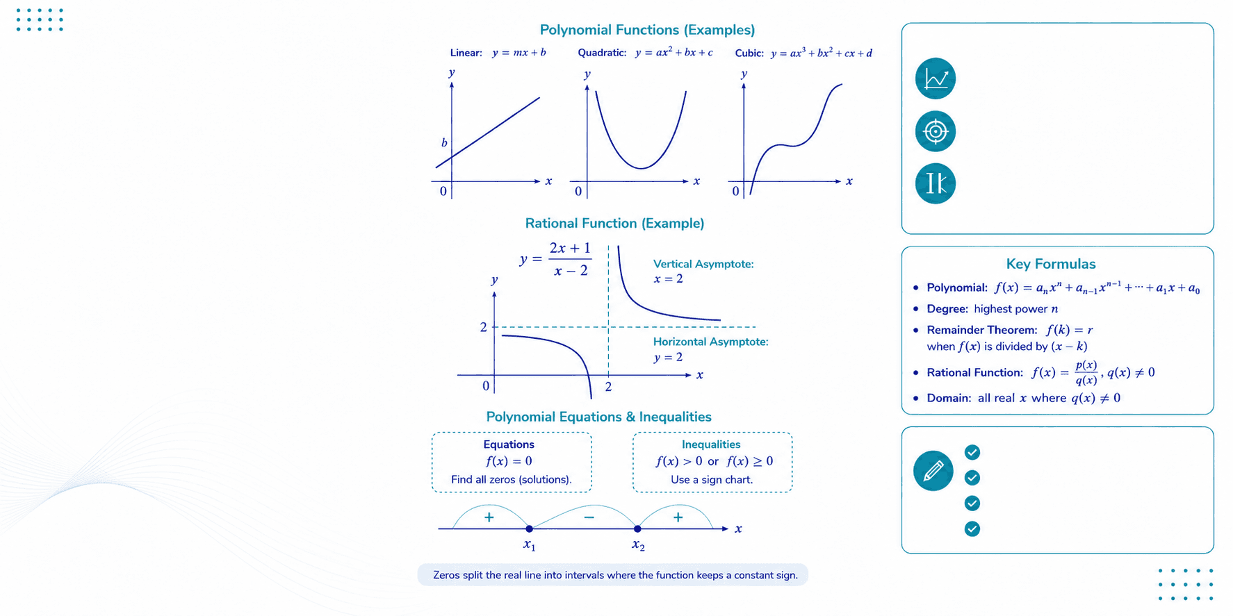
Polynomial and Rational Functions
Investigating the properties of polynomial and rational functions, and mastering polynomial equations and inequalities.
Key Concepts
On Your Worksheet
Graph and label key features.
Find zeros and intervals of increase/decrease.
Solve polynomial equations and inequalities.
Identify asymptotes and domain.
End Behaviour
Determined by the leading term and degree.
Zeros (x-intercepts)
Found by solving f(x)=0f(x)=0f(x)=0.
Asymptotes
Vertical, horizontal, or slant; describe long-term behaviour.

Trigonometry
Exploring trigonometric functions and developing techniques for applying these concepts.
Key Concepts
On Your Worksheet
Trigonometric Functions
Periodic functions that model cycles and waves.
Right Triangle Ratios
Relate the lengths of sides to acute angles.
Unit Circle
Connects angles in standard position to (cosθ,sinθ)
Applications
Used in real-world contexts including measurement, modeling, and problem-solving.
✓ Graph and analyze trig functions.
✓ Solve right triangle problems.
✓ Apply sine and cosine laws.
✓ Solve real-world trigonometry problems.

Exponential and Logarithmic Functions
Learning the properties of exponential and logarithmic functions and solving equations involving them.
Key Concepts
On Your Worksheet
Graph exponential growth and decay functions.
Graph logarithmic functions and identify asymptotes, domain, and range.
Apply transformation rules.
Solve exponential and logarithmic equations.
Exponential Functions
Model growth and decay processes.
Logarithmic Functions
Are inverses of exponential functions.

Combining Functions
Developing techniques for combining different types of functions and broadening understanding of rates of change.
Compose Functions
Combine functions by substitution.
Combine and Transform
Use combinations, sums, products, quotients, and transformations.
Rates of Change
Understand how combining functions affects the rate of change.
Domain Awareness
Check the domain after combining functions.
Find and simplify compositions.
Combine functions using +, −, ×, and ÷.
Graph and explore combined functions.
Determine and organize rates of change.
Identify domains and restrictions.
UNIT
1
UNIT
1
Students explore the graphs, end behaviors, and key properties of power and polynomial functions. Core concepts include the factor and remainder theorems, synthetic/long division, and solving polynomial equations and inequalities,
Students explore the graphs, end behaviors, and key properties of power and polynomial functions. Core concepts include the factor and remainder theorems, synthetic/long division, and solving polynomial equations and inequalities,
P(x) = anxn + ⋯ + a1x + a0
where an ≠ 0 and n is a non-negative integer.
The degree n determines how the graph extends as x approaches positive and negative infinity.
When P(x) is divided by (x − c), the remainder is P(c).
Example:
P(x) = 2x3 − 5x + 1
Divide by (x − 2):
Remainder = P(2)
= 2(2)3 − 5(2) + 1
= 16 − 10 + 1 = 7
(x − c) is a factor of P(x) if and only if P(c) = 0.
Example:
P(x) = x3 − 2x2 − x + 2
Test c = 1: P(1) = 1 − 2 − 1 + 2 = 0
Since P(1) = 0, (x − 1) is a factor.
Any rational root pq (in lowest terms) must have p a factor of a0 and q a factor of an.
Possible rational roots:
Takeaway: Use these theorems to test values, find factors, and identify possible rational roots before factoring or solving polynomial equations.
A rational function is any function that can be written as
where P(x) and Q(x) are polynomials and Q(x) ≠ 0.
Vertical asymptotes occur at values of x where
Q(x) = 0
and P(x) is not zero at the same x.
!These are values the function approaches but is undefined.
Determine by comparing degrees of P(x) and Q(x).
| Compare degrees | Horizontal asymptote |
|---|---|
| deg(P) < deg(Q) | y = 0 |
| deg(P) = deg(Q) | y = leading coeff. of P(x)leading coeff. of Q(x) |
| deg(P) > deg(Q) | No horizontal asymptote |
f(x) = 2x2 + 1x2 − 4 = 2x2 + 1(x − 2)(x + 2)
Set denominator factors equal to zero:
x − 2 = 0 ⇒ x = 2
x + 2 = 0 ⇒ x = −2
Vertical asymptotes: x = 2 and x = −2
Degrees are equal (2 and 2), so the horizontal asymptote is the ratio of leading coefficients.
y = 21 = 2
Horizontal asymptote: y = 2
x ≠ −2, 2
Graph sketch
UNIT
3
UNIT
3
Students delve into the inverse relationship between exponential and logarithmic expressions. Units cover logarithm laws, solving complex exponential and logarithmic equations, and using these functions to model real-world growth and decay (such as compound interest or pH levels)
Students delve into the inverse relationship between exponential and logarithmic expressions. Units cover logarithm laws, solving complex exponential and logarithmic equations, and using these functions to model real-world growth and decay (such as compound interest or pH levels)
Students delve into the inverse relationship between exponential and logarithmic expressions. Units cover logarithm laws, solving complex exponential and logarithmic equations, and using these functions to model real-world growth and decay (such as compound interest or pH levels)
Exponential functions have the form f(x) = a · bx.
Exponential models change at a rate proportional to the current value.
b > 1
0 < b < 1
Exponential growth models compound interest.
A = P(1 + rn)nt
Key idea: Exponential functions model situations where quantities grow or decay by a constant factor over equal intervals.
Definition: A logarithm is the inverse of an exponential function.
For a base b > 0,
b ≠ 1, and
x > 0:
logb(x) = y iff by = x
Logarithms convert multiplication into addition and powers into products, making them essential for solving equations and modelling growth and decay.
logb(xy) = logb(x) + logb(y)
The log of a product equals the sum of the logs.
logb(xy) = logb(x) − logb(y)
The log of a quotient equals the difference of the logs.
logb(xn) = n · logb(x)
The log of a power equals the exponent times the log.
log(5x+1) = log(12)
(x + 1) log(5) = log(12)
x = log(12)log(5) − 1≈ 0.544
Any log base > 0 and ≠ 1 can be used. (Commonly, base 10 or e.)
UNIT
2
UNIT
2
This unit bridges basic right-angle trigonometry with periodic wave functions. Students work with radian measure, the unit circle, and trigonometric ratios (including cosecant, secant, and cotangent). It also emphasizes transforming trigonometric graphs and solving basic trigonometric identities
This unit bridges basic right-angle trigonometry with periodic wave functions. Students work with radian measure, the unit circle, and trigonometric ratios (including cosecant, secant, and cotangent). It also emphasizes transforming trigonometric graphs and solving basic trigonometric identities
This unit bridges basic right-angle trigonometry with periodic wave functions. Students work with radian measure, the unit circle, and trigonometric ratios (including cosecant, secant, and cotangent). It also emphasizes transforming trigonometric graphs and solving basic trigonometric identities
Any point on the unit circle is (cos θ, sin θ).
180° = π radians.
Angles can be greater than 360° or negative.
sin2 θ + cos2 θ = 1
Radian measure uses arc length on a unit circle (radius 1): s = rθ = θ. This is the standard unit in calculus.
Radian measure is essential for higher-level calculus.
y = a · sin(b(x − c)) + d
= |a|
Vertical stretch by |a|. Reflect over the midline if a < 0.
= 2πb
Horizontal compression if b > 1; stretch if 0 < b < 1.
= c
Shift right c if c > 0, left |c| if c < 0.
= d
Shift up d if d > 0, down |d| if d < 0.
y = 3 sin(2(x − π4)) + 1
sin2θ + cos2θ = 1
Used to simplify expressions involving sine and cosine.
sin(α ± β) = sinα cosβ ± cosα sinβ
cos(α ± β) = cosα cosβ ∓ sinα sinβ
Meet Our Tutors
Meet Our Tutors
Reviews
Reviews

Rami Alzaytavi
B.ENG. Software Engineer

Yacoob Kathrada
Bsc. Biomedical

Maya Al Khowjeh
B.Tech. Civil Engineering

Taha Arafat
Msc. Pharmacology

Jawad Qourshah
B.ENG. Mechanical Engineering

Manish Bahat
M.ENG. Mechanical Engineering

Oubada Al Tarabishi
M.ENG. Electrical Engineering

Ahmad Dawood
MSc. Computer Science
Rami Alzaytavi
B.ENG. Software Engineer
Yacoob Kathrada
Bsc. Biomedical
Maya Al Khowjeh
B.Tech. Civil Engineering
Taha Arafat
Msc. Pharmacology
Jawad Qourshah
B.ENG. Mechanical Engineering
Manish Bahat
M.ENG. Mechanical Engineering
Oubada Al Tarabishi
M.ENG. Electrical Engineering
Ahmad Dawood
MSc. Computer Science
UNIT
4
UNIT
4
Teaches you how to create new functions by manipulating or nesting existing ones. This involves two main concepts: arithmetic operations and composition.
Combining functions means creating new functions from existing ones. These operations act on the output values of the functions at the same input x. Composition (f ∘ g) substitutes one function into another.
(f + g)(x) = f(x) + g(x)
Add the output values.
(f − g)(x) = f(x) − g(x)
Subtract the output values.
(f · g)(x) = f(x)g(x)
Multiply the output values.
(fg)(x) = f(x)g(x)
Divide the output values; requires g(x) ≠ 0.
(f ∘ g)(x) = f(g(x))
Substitute g(x) into f(x); mind the domain.
The resulting function is only defined for x where every step
makes sense.
Be especially careful with division (denominator ≠ 0) and composition
(inputs to the inner function must be valid).
Let f(x) = √x
and g(x) = x2 − 1.
Find the composition (f ∘ g)(x).
(f ∘ g)(x) = f(g(x)) = √x2 − 1
For the square root to be defined, x2 − 1 ≥ 0 So, x ≤ −1 or x ≥ 1.
Domain: (−∞, −1] ∪ [1, ∞)
FAQ
Is Advanced Functions Hard?

What is MHF4U?
MHF4U, MCV4U or MDM4U, which should I take?
Is Advanced Functions harder than Calculus?
Is Advanced Functions precalculus?
Is Advanced Functions easier than Grade 11 Functions?
Do you offer Advanced Functions tutoring online?
How do I get started?
Contact us


Grade 12 Advanced Functions; Prerequisite for Calculus & Vectors (MCV4U)
Grade 12 Advanced Functions; Prerequisite for Calculus & Vectors (MCV4U)
Grade 12 Advanced Functions; Prerequisite for Calculus & Vectors (MCV4U)
Build the strong foundation required for elite engineering programs. Expert One-on-One tutoring for the Ontario Grade 12 University Preparation Advanced Functions (MHF4U) curriculum.
Build the strong foundation required for elite engineering programs. Expert One-on-One tutoring for the Ontario Grade 12 University Preparation Advanced Functions (MHF4U) curriculum.
Build the strong foundation required for elite engineering programs. Expert One-on-One tutoring for the Ontario Grade 12 University Preparation Advanced Functions (MHF4U) curriculum.
100% Money-Back Guarantee on your first session.
100% Money-Back Guarantee on your first session.
Where Our Students Go
Where Our Students Go
Where Our Students Go





Coming Soon!
Review the major concepts taught throughout your course in one organized resource. The course review breaks challenging topics into smaller, understandable sections and provides clear examples showing how important concepts are applied.
✓ Polynomials and Rational Functions
✓ Trigonometry
✓ Exponential and Logarithmic Functions
✓ Combining Functions
✓ Core course topics and foundational concepts
✓ Clear explanations supported by worked examples
✓ Common mistakes and strategies for avoiding them
✓ Important skills needed for MHF4U
✓ Practice questions organized by course topic

What the Course
Review Includes
Topics Covered
Coming Soon!
Prepare for tests and final assessments with realistic, course-aligned practice exams. Each exam covers the major topics taught throughout the course, with detailed answer explanations that help students understand concepts, apply their knowledge, and learn from mistakes.
Students can use the practice exams to become familiar with different question formats, review challenging units, improve time management, and determine which concepts require additional preparation.

✓ Full-length practice exams
✓ Course-aligned and exam-style questions
✓ Questions from all major MHF4U topics
✓ Detailed step-by-step solution guides
✓ Focused review of mistakes and weaker areas
Coming Soon!
Identify a student’s current strengths, foundational learning gaps, and course-specific areas of difficulty. The diagnostic assessment evaluates understanding across major course topics and provides students with a clearer starting point for future review or tutoring.

The results can help Fit Minds Academy create a more personalized learning plan focused on the concepts and problem types requiring the most attention.
✓ Identify current course strengths
✓ Detect gaps in foundational Math knowledge
✓ Recognize challenging topics and question types
✓ Determine which skills require further practice
✓ Receive recommended next steps for improvement
Fit Minds Academy provides personalized 1-on-1 tutoring for high school students pursuing engineering programs and university students tackling challenging engineering courses. Our support covers math, physics, chemistry, calculus, statics, dynamics, thermodynamics, fluid mechanics, strength of materials, and other core engineering subjects.
Courses:

High School Courses
Support for Ontario high school students building the math and science foundation needed for future engineering programs.
Courses:

First-Year Engineering Courses
One-on-One private tutoring for core courses taken by every first years engineering student
Courses:

Advanced Engineering Courses
Course-specific tutoring for technical courses that require stronger applied problem-solving.

Personalized 1-on-1 Tutoring
Every student has different strengths, learning gaps, and academic goals. Each tutoring session is tailored to the student’s course, current level, pace, and areas requiring additional support. Lessons focus on the exact concepts and problem types the student needs to understand.
Carefully Matched Tutors for Every Student
Students are matched with tutors based on their course, academic level, subject requirements, learning needs, and availability. Many of our tutors are engineers or technical professionals who understand both the course material and its practical applications.
Ontario Curriculum and Engineering-Focused Support
Our high school tutoring follows the Ontario curriculum and supports the math and science prerequisites required for engineering, science, and technology programs. We also tutor first-year and upper-year university courses, including calculus, physics, linear algebra, programming, thermodynamics, fluid mechanics, and strength of materials.
More than Homework Help
Our tutoring goes beyond completing assignments or memorizing formulas. Students receive clear explanations, structured practice, and step-by-step problem-solving support designed to strengthen understanding and prepare them for quizzes, tests, exams, university courses, and future engineering studies.
Flexible Hourly Tutoring
$85
Per Hour
Pay-As-You-Go Plan, Billed Biweekly
✓ Sessions from the comfort of your home
✓ Access to Fit Minds Discord server
✓ Personalised sessions to suit you
✓ We teach your course material
✓ Resources (course notes, practice tests, and videos)
10-hour Prepaid Plan
$800
Per 10 Hours
$80 per hour - Save $50
✓ Sessions from the comfort of your home
✓ Access to Fit Minds Discord server
✓ Personalised sessions to suit you
✓ We teach your course material
✓ Resources (course notes, practice tests, and videos)
Not Sure Which Option Is Right?
Speak with Fit Minds Academy and find the Advanced Functions tutoring plan that best matches the student’s current course needs and academic goals.


Pricing
Pricing
Pricing
Rami Alzaytavi
B.ENG. Software Engineer
Yacoob Kathrada
Bsc. Biomedical
Maya Al Khowjeh
B.Tech. Civil Engineering
Taha Arafat
Msc. Pharmacology
Jawad Qourshah
B.ENG. Mechanical Engineering
Manish Bahat
M.ENG. Mechanical Engineering
Oubada Al Tarabishi
M.ENG. Electrical Engineering
Ahmad Dawood
MSc. Computer Science
Review the major concepts taught throughout your course in one organized resource. The course review breaks challenging topics into smaller, understandable sections and provides clear examples showing how important concepts are applied.
✓ Core course topics and foundational concepts
✓ Clear explanations supported by worked examples
✓ Common mistakes and strategies for avoiding them
✓ Important skills needed for MHF4U
✓ Practice questions organized by course topic

What the Course
Review Includes
Topics Covered
Coming Soon!
✓ Polynomials and Rational Functions
✓ Trigonometry
✓ Exponential and Logarithmic Functions
✓ Combining Functions
Coming Soon!
Prepare for tests and final assessments with realistic, course-aligned practice exams. Each exam covers the major topics taught throughout the course, with detailed answer explanations that help students understand concepts, apply their knowledge, and learn from mistakes.
Students can use the practice exams to become familiar with different question formats, review challenging units, improve time management, and determine which concepts require additional preparation.
✓ Full-length practice exams
✓ Course-aligned and exam-style questions
✓ Questions from all major MHF4U topics
✓ Detailed step-by-step solution guides
✓ Focused review of mistakes and weaker areas
Identify a student’s current strengths, foundational learning gaps, and course-specific areas of difficulty. The diagnostic assessment evaluates understanding across major course topics and provides students with a clearer starting point for future review or tutoring.
The results can help Fit Minds Academy create a more personalized learning plan focused on the concepts and problem types requiring the most attention.
✓ Identify current course strengths
✓ Detect gaps in foundational Math knowledge
✓ Recognize challenging topics and question types
✓ Determine which skills require further practice
✓ Receive recommended next steps for improvement
Coming Soon!
Fit Minds Academy provides personalized 1-on-1 tutoring for high school students pursuing engineering programs and university students tackling challenging engineering courses. Our support covers math, physics, chemistry, calculus, statics, dynamics, thermodynamics, fluid mechanics, strength of materials, and other core engineering subjects.
Courses:
High School Courses
Support for Ontario high school students building the math and science foundation needed for future engineering programs.
Courses:
First-Year Engineering Courses
One-on-One private tutoring for core courses taken by every first years engineering student
Courses:
Advanced Engineering Courses
Course-specific tutoring for technical courses that require stronger applied problem-solving.
Personalized 1-on-1 Tutoring
Every student has different strengths, learning gaps, and academic goals. Each tutoring session is tailored to the student’s course, current level, pace, and areas requiring additional support. Lessons focus on the exact concepts and problem types the student needs to understand.
Carefully Matched Tutors for Every Student
Students are matched with tutors based on their course, academic level, subject requirements, learning needs, and availability. Many of our tutors are engineers or technical professionals who understand both the course material and its practical applications.
Ontario Curriculum and Engineering-Focused Support
Our high school tutoring follows the Ontario curriculum and supports the math and science prerequisites required for engineering, science, and technology programs. We also tutor first-year and upper-year university courses, including calculus, physics, linear algebra, programming, thermodynamics, fluid mechanics, and strength of materials.
More than Homework Help
Our tutoring goes beyond completing assignments or memorizing formulas. Students receive clear explanations, structured practice, and step-by-step problem-solving support designed to strengthen understanding and prepare them for quizzes, tests, exams, university courses, and future engineering studies.
Flexible Hourly Tutoring
$85
Per Hour
Pay-As-You-Go Plan, Billed Biweekly
✓ Sessions from the comfort of your home
✓ Access to Fit Minds Discord server
✓ Personalised sessions to suit you
✓ We teach your course material
✓ Resources (course notes, practice tests, and videos)
10-hour Prepaid Plan
$800
Per 10 Hours
$80 per hour - Save $50
✓ Sessions from the comfort of your home
✓ Access to Fit Minds Discord server
✓ Personalised sessions to suit you
✓ We teach your course material
✓ Resources (course notes, practice tests, and videos)
Not Sure Which Option Is Right?
Speak with Fit Minds Academy and find the Advanced Functions tutoring plan that best matches the student’s current course needs and academic goals.
Contact us
Contact us
Flexible Hourly Tutoring
$85
Per Hour
Pay-As-You-Go Plan, Billed Biweekly
✓ Sessions from the comfort of your home
✓ Access to Fit Minds Discord server
✓ Personalised sessions to suit you
✓ We teach your course material
✓ Resources (course notes, practice tests, and videos)
10-hour Prepaid Plan
$800
Per 10 Hours
$80 per hour - Save $50
✓ Sessions from the comfort of your home
✓ Access to Fit Minds Discord server
✓ Personalised sessions to suit you
✓ We teach your course material
✓ Resources (course notes, practice tests, and videos)
Not Sure Which Option Is Right?
Speak with Fit Minds Academy and find the Advanced Functions tutoring plan that best matches the student’s current course needs and academic goals.
Personalized 1-on-1 Tutoring
Every student has different strengths, learning gaps, and academic goals. Each tutoring session is tailored to the student’s course, current level, pace, and areas requiring additional support. Lessons focus on the exact concepts and problem types the student needs to understand.
Carefully Matched Tutors for Every Student
Students are matched with tutors based on their course, academic level, subject requirements, learning needs, and availability. Many of our tutors are engineers or technical professionals who understand both the course material and its practical applications.
Ontario Curriculum and Engineering-Focused Support
Our high school tutoring follows the Ontario curriculum and supports the math and science prerequisites required for engineering, science, and technology programs. We also tutor first-year and upper-year university courses, including calculus, physics, linear algebra, programming, thermodynamics, fluid mechanics, and strength of materials.
More than Homework Help
Our tutoring goes beyond completing assignments or memorizing formulas. Students receive clear explanations, structured practice, and step-by-step problem-solving support designed to strengthen understanding and prepare them for quizzes, tests, exams, university courses, and future engineering studies.
Reviews
Fit Minds Academy provides personalized 1-on-1 tutoring for high school students pursuing engineering programs and university students tackling challenging engineering courses. Our support covers math, physics, chemistry, calculus, statics, dynamics, thermodynamics, fluid mechanics, strength of materials, and other core engineering subjects.
Courses:
High School Courses
Support for Ontario high school students building the math and science foundation needed for future engineering programs.
Courses:
First-Year Engineering Courses
One-on-One private tutoring for core courses taken by every first years engineering student
Courses:
Advanced Engineering Courses
Course-specific tutoring for technical courses that require stronger applied problem-solving.
Review the major concepts taught throughout your course in one organized resource. The course review breaks challenging topics into smaller, understandable sections and provides clear examples showing how important concepts are applied.
✓ Core course topics and foundational concepts
✓ Clear explanations supported by worked examples
✓ Common mistakes and strategies for avoiding them
✓ Important skills needed for MHF4U
✓ Practice questions organized by course topic

What the Course
Review Includes
Topics Covered
Coming Soon!
✓ Polynomials and Rational Functions
✓ Trigonometry
✓ Exponential and Logarithmic Functions
✓ Combining Functions
Prepare for tests and final assessments with realistic, course-aligned practice exams. Each exam covers the major topics taught throughout the course, with detailed answer explanations that help students understand concepts, apply their knowledge, and learn from mistakes.
Students can use the practice exams to become familiar with different question formats, review challenging units, improve time management, and determine which concepts require additional preparation.
✓ Full-length practice exams
✓ Course-aligned and exam-style questions
✓ Questions from all major MHF4U topics
✓ Detailed step-by-step solution guides
✓ Focused review of mistakes and weaker areas
Coming Soon!
✓ Full-length practice exams
✓ Course-aligned and exam-style questions
✓ Questions from all major MHF4U topics
✓ Detailed step-by-step solution guides
✓ Focused review of mistakes and weaker areas
Identify a student’s current strengths, foundational learning gaps, and course-specific areas of difficulty. The diagnostic assessment evaluates understanding across major course topics and provides students with a clearer starting point for future review or tutoring.
The results can help Fit Minds Academy create a more personalized learning plan focused on the concepts and problem types requiring the most attention.
✓ Identify current course strengths
✓ Detect gaps in foundational Math knowledge
✓ Recognize challenging topics and question types
✓ Determine which skills require further practice
✓ Receive recommended next steps for improvement
Coming Soon!
UNIT
4
Teaches you how to create new functions by manipulating or nesting existing ones. This involves two main concepts: arithmetic operations and composition.
Combining functions means creating new functions from existing ones. These operations act on the output values of the functions at the same input x. Composition (f ∘ g) substitutes one function into another.
(f + g)(x) = f(x) + g(x)
Add the output values.
(f − g)(x) = f(x) − g(x)
Subtract the output values.
(f · g)(x) = f(x)g(x)
Multiply the output values.
(fg)(x) = f(x)g(x)
Divide the output values; requires g(x) ≠ 0.
(f ∘ g)(x) = f(g(x))
Substitute g(x) into f(x); mind the domain.
The resulting function is only defined for x where every step
makes sense.
Be especially careful with division (denominator ≠ 0) and composition
(inputs to the inner function must be valid).
Let f(x) = √x
and g(x) = x2 − 1.
Find the composition (f ∘ g)(x).
(f ∘ g)(x) = f(g(x)) = √x2 − 1
For the square root to be defined, x2 − 1 ≥ 0 So, x ≤ −1 or x ≥ 1.
Domain: (−∞, −1] ∪ [1, ∞)
UNIT
1
Students explore the graphs, end behaviors, and key properties of power and polynomial functions. Core concepts include the factor and remainder theorems, synthetic/long division, and solving polynomial equations and inequalities,
Any point on the unit circle is (cos θ, sin θ).
180° = π radians.
Angles can be greater than 360° or negative.
sin2 θ + cos2 θ = 1
Radian measure uses arc length on a unit circle (radius 1): s = rθ = θ. This is the standard unit in calculus.
Radian measure is essential for higher-level calculus.
P(x) = anxn + ⋯ + a1x + a0
where an ≠ 0 and n is a non-negative integer.
The degree n determines how the graph extends as x approaches positive and negative infinity.
When P(x) is divided by (x − c), the remainder is P(c).
Example:
P(x) = 2x3 − 5x + 1
Divide by (x − 2):
Remainder = P(2)
= 2(2)3 − 5(2) + 1
= 16 − 10 + 1 = 7
(x − c) is a factor of P(x) if and only if P(c) = 0.
Example:
P(x) = x3 − 2x2 − x + 2
Test c = 1: P(1) = 1 − 2 − 1 + 2 = 0
Since P(1) = 0, (x − 1) is a factor.
Any rational root pq (in lowest terms) must have p a factor of a0 and q a factor of an.
Possible rational roots:
Takeaway: Use these theorems to test values, find factors, and identify possible rational roots before factoring or solving polynomial equations.
A rational function is any function that can be written as
where P(x) and Q(x) are polynomials and Q(x) ≠ 0.
Vertical asymptotes occur at values of x where
Q(x) = 0
and P(x) is not zero at the same x.
!These are values the function approaches but is undefined.
Determine by comparing degrees of P(x) and Q(x).
| Compare degrees | Horizontal asymptote |
|---|---|
| deg(P) < deg(Q) | y = 0 |
| deg(P) = deg(Q) | y = leading coeff. of P(x)leading coeff. of Q(x) |
| deg(P) > deg(Q) | No horizontal asymptote |
f(x) = 2x2 + 1x2 − 4 = 2x2 + 1(x − 2)(x + 2)
Set denominator factors equal to zero:
x − 2 = 0 ⇒ x = 2
x + 2 = 0 ⇒ x = −2
Vertical asymptotes: x = 2 and x = −2
Degrees are equal (2 and 2), so the horizontal asymptote is the ratio of leading coefficients.
y = 21 = 2
Horizontal asymptote: y = 2
x ≠ −2, 2
Graph sketch
Polynomial and Rational Functions
Investigating the properties of polynomial and rational functions, and mastering polynomial equations and inequalities.
Key Concepts
On Your Worksheet
Graph and label key features.
Find zeros and intervals of increase/decrease.
Solve polynomial equations and inequalities.
Identify asymptotes and domain.
End Behaviour
Determined by the leading term and degree.
Zeros (x-intercepts)
Found by solving f(x)=0f(x)=0f(x)=0.
Asymptotes
Vertical, horizontal, or slant; describe long-term behaviour.
Trigonometry
Exploring trigonometric functions and developing techniques for applying these concepts.
Trigonometric Functions
Periodic functions that model cycles and waves.
Right Triangle Ratios
Relate the lengths of sides to acute angles.
Unit Circle
Connects angles in standard position to (cosθ,sinθ)
Applications
Used in real-world contexts including measurement, modeling, and problem-solving.
✓ Graph and analyze trig functions.
✓ Solve right triangle problems.
✓ Apply sine and cosine laws.
✓ Solve real-world trigonometry problems.
Key Concepts
On Your Worksheet
Exponential and Logarithmic Functions
Learning the properties of exponential and logarithmic functions and solving equations involving them.
Key Concepts
On Your Worksheet
Graph exponential growth and decay functions.
Graph logarithmic functions and identify asymptotes, domain, and range.
Apply transformation rules.
Solve exponential and logarithmic equations.
Exponential Functions
Model growth and decay processes.
Logarithmic Functions
Are inverses of exponential functions.

Combining Functions
Developing techniques for combining different types of functions and broadening understanding of rates of change.
Compose Functions
Combine functions by substitution.
Combine and Transform
Use combinations, sums, products, quotients, and transformations.
Rates of Change
Understand how combining functions affects the rate of change.
Domain Awareness
Check the domain after combining functions.
Find and simplify compositions.
Combine functions using +, −, ×, and ÷.
Graph and explore combined functions.
Determine and organize rates of change.
Identify domains and restrictions.